How to Prepare a PSLF User-Defined Model: EPCL, Files, and Run Modes

CAISO’s Cluster 16 process put PSLF user-defined models in focus. The initial GRIP notice said non-synchronous generator applicants would need to upload a PSLF-generated user-defined model with responses similar to the generic model. That created a practical gap for teams whose available model was a parameterized WECC generic-library model, but who did not yet have a user-defined model ready.

CAISO later said Cluster 16 applicants without a user-defined model could submit their parameterized generic-library RMS positive-sequence model in GRIP’s user-defined-model field to complete the application. CAISO also published a temporary placeholder that delays the tariff requirement; it says applicants will be notified when the model is due and must be validated. These are interim, Cluster 16-specific instructions, not a permanent replacement for a user-defined model, so confirm CAISO’s current directions for your project (initial Cluster 16 notice, modified model requirement, temporary placeholder).

Before starting a model for a project, confirm the current submission requirements, accepted interface and format, and validation evidence expected by the relevant transmission provider. A user-defined model also needs to be tested against the equipment behavior it is intended to represent; compiling successfully is only one step in that process.

This guide focuses on the first step: understanding EPCL, the files in a dynamic study, and the modes PSLF calls before writing more advanced model logic.

The usual building blocks

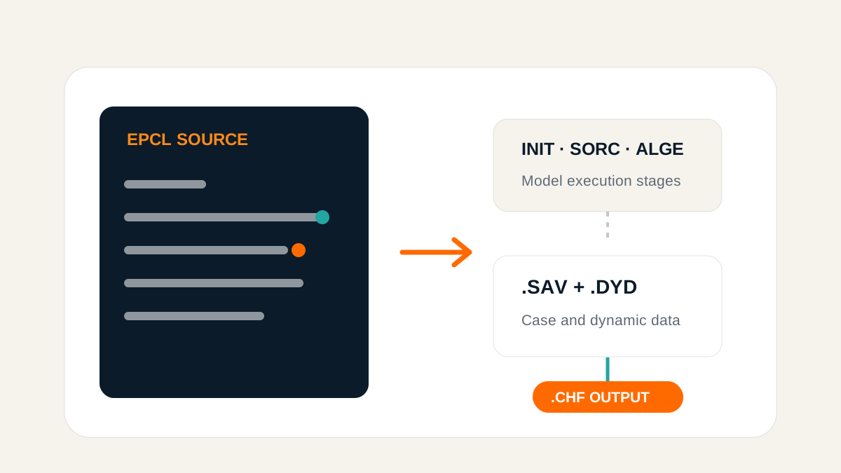
EPCL is PSLF’s built-in language for model logic and automation. A dynamic-model source file is commonly written as a .p file. It is then compiled or processed for use by PSLF according to the workflow supported by the installed release. Keep the source readable, comment the purpose of each calculation, and separate model parameters from temporary calculation values.

Numeric and text variables

EPCL uses different prefixes to make the intended variable type clear:

Prefix	General use	Example idea
@	Numeric variable	@error for a numeric difference or @count for an integer-like counter
$	Character or string variable	$label for a text label or $status for a short message

Use a numeric variable for values that take part in arithmetic, comparisons, or equations. Use a string variable for labels and text. Give variables names that describe their purpose, such as @current_error or @voltage_reference, rather than relying on temporary names like @x1 and @x2. Follow the naming, declaration, scope, and array rules in the EPCL reference shipped with your PSLF version; the prefixes alone do not determine how a variable is initialized or shared.

Before writing model equations, sketch the inputs, states, outputs, units, and limits. This makes it easier to see which values are parameters, which must be integrated as states, and which are only intermediate calculations.

Understand the model execution modes

PSLF calls different parts of a dynamic model at different stages of the simulation. The familiar EPCL model modes divide that work into responsibilities:

Mode	General responsibility
INIT	Initialize model states and outputs from the solved operating point
SORC	Calculate the model’s electrical source or network-boundary quantities when it interfaces directly with the network
NTWK	Solve the network using the assembled injections; this is handled by the PSLF solution process
ALGE	Update algebraic or derived quantities that do not require state integration
RATE	Calculate derivatives of dynamic state variables for numerical integration
OUTP	Make selected values available to recorded output channels

The exact call sequence and which modes a model needs depend on its role and the PSLF release. For example, a controller that acts through another device may not calculate a direct network injection of its own. Use the model-writing reference for the installed version before relying on a particular sequence. Thinking in these stages helps keep initialization, network interaction, state updates, and recorded outputs from becoming one tangled calculation.

Define channels for debugging and review

The PSLF channel type field is four characters, and the code entered there is the identifier exported in the .chf file. Choose clear, unique names so that each trace is easy to recognize later. For temporary debug channels, use a numbered family such as DE01 and DE02, then keep a note of what each code represents.

PSLF models can keep algebraic quantities and persistent values in vN slots, while sN slots hold dynamic states that PSLF integrates over time. The model calculates each state’s derivative in the matching dsN slot during RATE. For example, v1 could hold an active-power reference, while s1 could hold the state of a low-pass filter on active power. Slot meanings are model-specific. The example source here uses V slots for its persistent values and diagnostics; it does not define S states.

In EPCL, set the channel name through channel_head[n].type. The channel header index matches the persistent model variable slot with the same number: channel_head[0] names the value stored in .v0, channel_head[1] names .v1, and so on. For example, in an EPCMOD model:

@active_power_error = @active_power_reference - @measured_active_power
epcmod[@mx].v0 = @active_power_error
channel_head[0].type = "DE01"

@voltage_error = @v_reference - @v_measured
epcmod[@mx].v2 = @voltage_error
channel_head[2].type = "DE02"

Here @active_power_error and @voltage_error are readable EPCL numeric variables. The .v0 and .v2 slots retain their values between model calls, while DE01 and DE02 give those outputs short names in the channel file. v1 remains available for the active-power reference in this illustration. Initialize any slots you use and check the existing .vN assignments before choosing a slot, so a debug trace does not overwrite another model value.

For each channel, record its units, base, sign convention, and expected range. Then compare the trace against a hand calculation or a simple test case. This catches errors such as mixing per-unit and physical values, reversing a sign, or updating a signal in a stage where it is not yet valid.

Know which file you are looking at

File	Typical role in a PSLF study
.p	EPCL source text used for model logic or automation
.dyd	Dynamic model data associated with devices in a case
.sav	Saved power-flow case used as a starting point for a study
.drw	Drawing file for the single-line diagram or another PSLF drawing
.chf	Recorded dynamic channels and their time-series values

A .sav is a saved network case, not the source code for a dynamic model. A .dyd supplies dynamic model records; it is read in the context of the relevant case and model definitions. A .drw is for the drawing view of a network, such as its single-line diagram. The .chf is the time-series result file produced by recording selected channels. These files describe different stages of a workflow and should not be treated as interchangeable copies of the same study.

A practical first workflow

1. Read the PSLF EPCL and dynamic-model manuals for your installed release.
2. Write down the model’s inputs, states, outputs, units, and limits.
3. Organize calculations by the mode that owns them: initialize, calculate network interaction, update algebraic values, calculate rates, and publish output.
4. Add a small set of output channels that lets you check the model’s behavior.
5. Test initialization and simple operating points before interpreting a complicated disturbance.
6. Review the recorded .chf channels and compare them with independent expectations.

Following this workflow gives you a starting point for a user-defined model and a .chf file containing the channels you chose to record. During model development, you may need to inspect many signals, including internal debug outputs. ESPlotter can read the binary .chf through the installed PSLF API and list its recorded channels; drag signals onto plots to inspect responses and compare variables before documenting the results. Download ESPlotter for Windows.